Nube de datos: left

Mostrando entradas con la etiqueta left_join. Mostrar todas las entradas

2020-05-01

Create a mini IMDb database in R

Introduction

In a previous post we showed how to extract movie info R info using the imdbapi package. In this post we will create a mini imdb database using the same package.

Solution

If we use the free version, the maximum number of requests per day is 1,000. We need to request an API key here.

First we need a vector containing the movie titles or the IMDbIDs (e.g.: for Vertigo the last section of the url https://www.imdb.com/title/tt0052357/, the string tt0052357. In our example we will use the list containing the results from the Sight and Sound 2012 poll of 846 critics, these are the films receiving at least 3 votes.

library(imdbapi)
library(data.table)
library(tidyverse)
sight_sound <- read.csv("https://sites.google.com/site/nubededatosblogspotcom/Sight&Sound2012-CriticsPoll.txt", stringsAsFactors = FALSE)
glimpse(sight_sound)

Observations: 588
Variables: 17
$ const                          "tt0052357", "tt0033467", "tt004643...
$ position                       1, 2, 3, 4, 5, 6, 7, 8, 9, 10, 11, ...
$ created                        "Thu Aug 16 07:42:05 2012", "Thu Au...
$ description                    NA, NA, NA, NA, NA, NA, NA, NA, NA,...
$ modified                       "Thu Aug 16 07:42:05 2012", "Thu Au...
$ Title                          "Vertigo", "Citizen Kane", "Tôkyô m...
$ Directors                      "Alfred Hitchcock", "Orson Welles",...
$ Title.type                     "Feature Film", "Feature Film", "Fe...
$ IMDb.Rating                    8.5, 8.5, 8.2, 8.0, 8.3, 8.3, 8.0, ...
$ PeacefulAnarchy.rated          10, 9, 10, 9, 9, 6, 6, 10, 8, 9, 6,...
$ Runtime..mins.                 128, 119, 136, 110, 94, 160, 119, 6...
$ Genres                         "mystery, romance, thriller", "dram...
$ Year                           1958, 1941, 1953, 1939, 1927, 1968,...
$ Num.Votes                      153502, 205699, 16219, 14872, 19188...
$ Release.Date..month.day.year.  "1958-05-09", "1941-05-01", "1953-1...
$ Id                             1, 2, 3, 4, 5, 6, 7, 8, 9, 10, 11, ...
$ URL                            "http://www.imdb.com/title/tt005235...

We use the function lapply to extract the info for all IMDbIDs.

tt <-
  lapply(sight_sound$const, function(x) {
    return(tryCatch(
      find_by_id(
        x,
        type = NULL,
        year_of_release = NULL,
        plot = "full",
        include_tomatoes = TRUE,
        api_key = "12345678"
      ),
      error = function(e)
        NULL
    ))
  })
df_sight_sound <- rbindlist(tt, fill = TRUE)
df_sight_sound$Ratings <- as.character(df_sight_sound$Ratings)
df_sight_sound <- as.data.frame(df_sight_sound)
df_sight_sound %>% distinct(imdbID) %>% summarise(n= n())

    n
1 586

After running the code some titles may be missing. In our examples, two title. We will repeat the process until obtain all of them.

# Checking missing titles
m <- subset(sight_sound, !(const %in% df_sight_sound$imdbID))$const 
m

[1] "tt0115751" "tt0032551"

Finally, we keep distinct titles removing duplicates.

df_sight_sound <- df_sight_sound %>% 
  filter(grepl("Internet",Ratings)) %>% 
  group_by(imdbID) %>% 
  distinct()

# A tibble: 588 x 26
# Groups:   imdbID [588]
   Title Year  Rated Released   Runtime Genre Director Writer Actors Plot 
                       
 1 Vert~ 1958  PG    1958-07-21 128 min Myst~ Alfred ~ "Alec~ James~ "Joh~
 2 Citi~ 1941  PG    1941-09-05 119 min Dram~ Orson W~ Herma~ Josep~ "A g~
 3 Toky~ 1953  NOT ~ 1972-03-13 136 min Drama Yasujir~ Kôgo ~ Chish~ An e~
 4 The ~ 1939  NOT ~ 1950-04-08 110 min Come~ Jean Re~ Jean ~ Nora ~ Avia~
 5 Sunr~ 1927  NOT ~ 1927-11-04 94 min  Dram~ F.W. Mu~ Carl ~ Georg~ "In ~
 6 2001~ 1968  G     1968-05-12 149 min Adve~ Stanley~ Stanl~ Keir ~ "\"2~
 7 The ~ 1956  PASS~ 1956-05-26 119 min Adve~ John Fo~ Frank~ John ~ Etha~
 8 Man ~ 1929  NOT ~ 1929-05-12 68 min  Docu~ Dziga V~ Dziga~ Mikha~ This~
 9 The ~ 1928  NOT ~ 1928-10-25 114 min Biog~ Carl Th~ Josep~ Maria~ The ~
10 8½    1963  NOT ~ 1963-06-25 138 min Drama Federic~ Feder~ Marce~ Guid~
# ... with 578 more rows, and 16 more variables: Language ,
#   Country , Awards , Poster , Ratings ,
#   Metascore , imdbRating , imdbVotes , imdbID ,
#   Type , DVD , BoxOffice , Production , Website ,
#   Response , totalSeasons

To export the final results as a csv:

write.csv(df_sight_sound, "df_sight_sound.csv", row.names = FALSE)

Extract movie info using the OMDb API in R

References

2019-08-25

How to rename suffixes when joining tables in dplyr

Problem

When joining two tables with dplyr, the suffixes .x and .y will be added to the non-joined duplicate variables to disambiguate them. In our example, to the column mpg: mpg.x y mpg.y. How can override these suffixes?

library(dplyr) 
left_join(mtcars, mtcars[, c("mpg", 'cyl')], by = c("cyl")) %>% head()

Output

  mpg.x cyl disp  hp drat   wt  qsec vs am gear carb mpg.y
1    21   6  160 110  3.9 2.62 16.46  0  1    4    4  21.0
2    21   6  160 110  3.9 2.62 16.46  0  1    4    4  21.0
3    21   6  160 110  3.9 2.62 16.46  0  1    4    4  21.4
4    21   6  160 110  3.9 2.62 16.46  0  1    4    4  18.1
5    21   6  160 110  3.9 2.62 16.46  0  1    4    4  19.2
6    21   6  160 110  3.9 2.62 16.46  0  1    4    4  17.8

Solution

We can pass the argument suffix, a character vector of length 2 with the desired names. In our example, mpg_original (suffix _original) and mpg_new (suffix_new).

left_join(mtcars, mtcars[,c("mpg","cyl")], 
              by = c("cyl"), 
              suffix = c("_original", "_new")) %>% head()

Output

  mpg_original cyl disp  hp drat   wt  qsec vs am gear carb mpg_new
1           21   6  160 110  3.9 2.62 16.46  0  1    4    4    21.0
2           21   6  160 110  3.9 2.62 16.46  0  1    4    4    21.0
3           21   6  160 110  3.9 2.62 16.46  0  1    4    4    21.4
4           21   6  160 110  3.9 2.62 16.46  0  1    4    4    18.1
5           21   6  160 110  3.9 2.62 16.46  0  1    4    4    19.2
6           21   6  160 110  3.9 2.62 16.46  0  1    4    4    17.8

References

2018-12-03

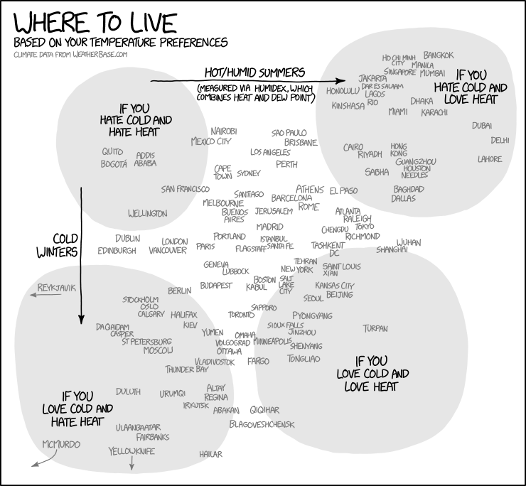
Dónde vivir en función de la temperatura (gráfico estilo xkcd)

Introducción

Hace aproximadamente un año, inspirados por el siguiente gráfico gráfico de xkcd, diferentes alternativas del mismo aparecieron en varios blogs, centradas generalmente en un país. El inicial de Maëlle Salmon para EUU, así como para España, Alemania, Países Bajos, Europa y Japón.

En primer lugar crearé mi versión para todo el mundo por continente. En segundo lugar para España incluyendo mapas con la ubicación de las ciudades.

Variables

En los gráficos y mapas vamos a emplear dos variables:

Temperatura media en invierno
Indice Humidex: wiki en español y en inglés.

Gráficos por continente

Creamos un gráfico para cada continente para evitar un apelotonamiento de ciudades. Dejamos la función facet_wrap, aunque cada gráfico está en un único panel, para obtener el subtítulo con el nombre del continente.

library(rvest)
library(tidyverse)
library(ggplot2)
library(ggrepel)
library(xkcd)
library(extrafont)
library(riem)

url <- "https://www.explainxkcd.com/wiki/index.php/1916:_Temperature_Preferences"
temp <- url %>% 
  read_html() %>% 
  html_node(xpath ='//*[@id="mw-content-text"]/div/table[2]') %>% 
  html_table()

# Para reproducir mismos resultados
set.seed(2015)

# Incluimos a Estambul dentro de Europa
temp <- temp %>% mutate(Continent = replace(Continent, City == "Istanbul", "Europe"))

# Bucle por continente
cont_list <- unique(temp$Continent)
plots <- list() # Guardamos gráficos en una lista
for (i in seq_along(cont_list)) { 
# Rangos de los ejes
rng <- temp %>% filter(Continent == cont_list[i])   
xrange <- c(floor(min(rng$Humidex, na.rm = TRUE)/10)*10, 
            ceiling(max(rng$Humidex, na.rm = TRUE)/10)*10)
yrange <- c(floor(min(rng$`Average low in coldest month (°C)`,na.rm = TRUE)/10)*10, 
            ceiling(max(rng$`Average low in coldest month (°C)`, na.rm = TRUE)/10)*10)
# Gráfico por continente
plot <- temp %>% filter(Continent == cont_list[i]) %>%
  ggplot(aes(Humidex, `Average low in coldest month (°C)`)) +
  geom_point() +
  geom_text_repel(aes(label = City),
                  family = "xkcd",
                  max.iter = 50000) +
  facet_wrap( ~ Continent) + 
  ggtitle("Where to live\nbased on your temperature preferences",
          subtitle = "Data source: www.explainxkcd.com") +
  xlab("Humidex: summer heat and humidity") +
  ylab("Avg. winter temperature in Celsius") +
  xkcdaxis(xrange = xrange,
           yrange = yrange) +
  scale_x_continuous(breaks = seq(min(xrange), max(xrange), by = 10)) +
  scale_y_continuous(breaks = seq(min(yrange), max(yrange), by = 10)) +
  theme_xkcd() +
  theme(text = element_text(size = 16, family = "xkcd")) +
  theme(text = element_text(size = 16, family = "xkcd"))
plots[[i]] = plot
print(plot) 
}

España

# Importamos nombres de aeoropuertos españoles
url <- "https://es.wikipedia.org/wiki/Anexo:Aeropuertos_de_Espa%C3%B1a"
spain_airports <- url %>% 
  read_html() %>% 
  html_node(xpath ='//*[@id="mw-content-text"]/div/table[1]') %>% 
  html_table()
spain_airports$aeropuertos <- str_extract(spain_airports$`Aeropuertos públicos`, "[^\\[]+")
# Editamos los nombres de los aeropueros manualmente
nombres <- read.csv("spain_airports_editados.csv")

# Temperaturas usando el paquete riem
summer_data <- map_df(riem_stations('ES__ASOS')$id, riem_measures,
                                date_start = "2018-06-01",
                                date_end = "2018-08-31")
winter_data <- map_df(riem_stations('ES__ASOS')$id, riem_measures,
                                date_start = "2017-12-01",
                                date_end = "2018-02-28")

# Conversión a grados centígrados
library(weathermetrics)
summer_data <- summer_data %>% 
                    mutate(tmpc = convert_temperature(tmpf,
                                                      old_metric = "f", 
                                                      new_metric = "c"),
                           dwpc = convert_temperature(dwpf,
                                                      old_metric = "f",
                                                      new_metric = "c"))
winter_data <- winter_data %>%
                     mutate(tmpc = convert_temperature(tmpf,
                               old_metric = "f",
                               new_metric = "c"),
                            dwpc = convert_temperature(dwpf, 
                               old_metric = "f",
                               new_metric = "c"))


# Cálculo de humidex
library(comf)
summer_data <- summer_data %>%
                    mutate(humidex = calcHumx(tmpc, relh)) %>% 
                   group_by(station, lon, lat) %>%
                   summarize(summer_avg_temp = mean(tmpc, na.rm = TRUE),
                      summer_humidex = mean(humidex, na.rm = TRUE))
winter_data <- winter_data %>%
                    group_by(station,lon, lat) %>%
                   summarize(winter_avg_temp = mean(tmpc, na.rm = TRUE))

# Unimos datos y nombres de aeropuertos
climate <- dplyr::left_join(winter_data, summer_data,
                             by = "station")
climate <- dplyr::left_join(climates, nombres)


# Gráfico
set.seed(2015)
xrange <- range(climate$summer_humidex)
yrange <- range(climate$winter_avg_temp)
climate %>% 
  ggplot(aes(summer_humidex, winter_avg_temp)) +
  geom_point() +
  geom_text_repel(aes(label = toupper(aeropuertos) ), 
                  family = "xkcd",
                  max.iter = 50000) +
  ggtitle("Where to live in Spain based on your temperature preferences",
          subtitle = "Data from airport weather stations 2017-2018") +
  xlab("Humidex: summer heat and humidity") +
  ylab("Avg. winter temperature in Celsius") +
  xkcdaxis(xrange = xrange,
           yrange = yrange) +
  theme_xkcd() +
  theme(text = element_text(size = 16, family = "xkcd")) +
  theme(text = element_text(size = 16, family = "xkcd"))

Mapas de España

Muestro dos tipos de gráfico. El invierno con una paleta basada en un color azul y el verano con la escala viridis. En este caso no disponemos de una tabla con las temperaturas, por lo que usamos el paquete riem (“R Iowa Environmental Mesonet”) creado por Maëlle Salmon que extrae la información de aquí.

Invierno

# Península
set.seed(2015)
climate_spain_map %>% 
  filter(lon > -10) %>% 
  ggplot(aes(lon, lat)) +
  geom_point(aes(color = winter_avg_temp), size = 3.5) +
  geom_text_repel(aes(label = aeropuertos),
                  family = "xkcd", size = 4.5,
                  max.iter = 50000) +
  geom_polygon(data = spain, aes(x = long, y = lat, group = group), 
               fill = NA, color = "black") +
  coord_map() +
  labs(title = "Avg. Winter Temperature in Spain",
       subtitle = "Data from Iowa Environment Mesonet 2017-2018",
       x = "", y = "") +
  theme_xkcd() +
  theme(axis.text.x=element_blank(),
        axis.ticks.x=element_blank(),
        axis.text.y=element_blank(),
        axis.ticks.y=element_blank())+
  scale_color_gradient(low = "#08306B")

# Canarias
canary <- map_data(map = "world", region = "Canary Islands")
climate_canary_map <- left_join(climates, lat_lon, by = "station")

set.seed(2015)
climate_canary_map %>% 
  filter(lon < -10) %>% 
  ggplot(aes(lon, lat)) +
  geom_point(aes(color = winter_avg_temp), size = 3.5) +
  geom_text_repel(aes(label = aeropuertos),
                  family = "xkcd", size = 4.5,
                  max.iter = 50000) +
  geom_polygon(data = canary, aes(x = long, y = lat, group = group), 
               fill = NA, color = "black") +
  coord_map() +
  labs(title = "Avg. Winter Temperature in Canary Islands",
       subtitle = "Data from Iowa Environment Mesonet 2017-2018",
       x = "", y = "") +
  theme_xkcd() +
   theme(axis.text.x=element_blank(),
        axis.ticks.x=element_blank(),
        axis.text.y=element_blank(),
        axis.ticks.y=element_blank()) +
  scale_color_gradient(low = "#08306B")

Verano

# Península
set.seed(2015)
climate_spain_map %>% 
  filter(lon > -10) %>% 
  ggplot(aes(lon, lat)) +
  geom_point(aes(color = summer_humidex), size = 3.5) +
  geom_text_repel(aes(label = aeropuertos),
                  family = "xkcd", size = 4.5,
                  max.iter = 50000) +
  geom_polygon(data = spain, aes(x = long, y = lat, group = group), 
               fill = NA, color = "black") +
  coord_map() +
  labs(title = "Avg. Summer Humidex in Spain",
       subtitle = "Data from Iowa Environment Mesonet 2017-2018",
       x = "", y = "") +
  theme_xkcd() +
  theme(axis.text.x=element_blank(),
        axis.ticks.x=element_blank(),
        axis.text.y=element_blank(),
        axis.ticks.y=element_blank()) +
    scale_color_viridis_c()

# Canarias
set.seed(2015)
climate_canary_map %>% 
  filter(lon < -10) %>% 
  ggplot(aes(lon, lat)) +
  geom_point(aes(color = summer_humidex), size = 3.5) +
  geom_text_repel(aes(label = aeropuertos),
                  family = "xkcd", size = 4.5,
                  max.iter = 50000) +
  geom_polygon(data = canary, aes(x = long, y = lat, group = group), 
               fill = NA, color = "black") +
  coord_map() +
  labs(title = "Avg. Summer Humidex in Canary Islands",
       subtitle = "Data from Iowa Environment Mesonet 2017-2018",
       x = "", y = "") +
  theme_xkcd() +
   theme(axis.text.x=element_blank(),
        axis.ticks.x=element_blank(),
        axis.text.y=element_blank(),
        axis.ticks.y=element_blank()) +
   scale_color_viridis_c()

Entradas relacionadas

2018-11-29

Crear una pequeña base de datos de IMDb con R

Introducción

En una entrada anterior usamos la OMDb API para extraer con R información sobre películas o series de televisión. En esta ocasión queremos crear una pequeña base datos con el mismo paquete imdbapi.

Solución

Empleamos el paquete imdbapi que nos permite extraer dicha información. Si utilizamos la versión gratuita, tendremos una limitación de 1.000 peticiones al día.

Lo primero que necesitamos es un vector con títulos de películas o de IMDbIDs (por ejemplo: para Vértigo la parte final de la dirección https://www.imdb.com/title/tt0052357/, la cadena tt0052357. En nuestro ejemplo usamos la encuesta de los críticos Sight & Sound de 2012, que contiene la columna const con dichos IMDbIDs .

library(imdbapi)
library(data.table)
library(tidyverse)
sight_sound <- read.csv("https://sites.google.com/site/nubededatosblogspotcom/Sight&Sound2012-CriticsPoll.txt", stringsAsFactors = FALSE)
glimpse(sight_sound)

Observations: 588
Variables: 17
$ const                          "tt0052357", "tt0033467", "tt004643...
$ position                       1, 2, 3, 4, 5, 6, 7, 8, 9, 10, 11, ...
$ created                        "Thu Aug 16 07:42:05 2012", "Thu Au...
$ description                    NA, NA, NA, NA, NA, NA, NA, NA, NA,...
$ modified                       "Thu Aug 16 07:42:05 2012", "Thu Au...
$ Title                          "Vertigo", "Citizen Kane", "Tôkyô m...
$ Directors                      "Alfred Hitchcock", "Orson Welles",...
$ Title.type                     "Feature Film", "Feature Film", "Fe...
$ IMDb.Rating                    8.5, 8.5, 8.2, 8.0, 8.3, 8.3, 8.0, ...
$ PeacefulAnarchy.rated          10, 9, 10, 9, 9, 6, 6, 10, 8, 9, 6,...
$ Runtime..mins.                 128, 119, 136, 110, 94, 160, 119, 6...
$ Genres                         "mystery, romance, thriller", "dram...
$ Year                           1958, 1941, 1953, 1939, 1927, 1968,...
$ Num.Votes                      153502, 205699, 16219, 14872, 19188...
$ Release.Date..month.day.year.  "1958-05-09", "1941-05-01", "1953-1...
$ Id                             1, 2, 3, 4, 5, 6, 7, 8, 9, 10, 11, ...
$ URL                            "http://www.imdb.com/title/tt005235...

Empleamos la función lapply para extraer la información de todos los IMDbIDs.

tt <-
  lapply(sight_sound$const, function(x) {
    return(tryCatch(
      find_by_id(
        x,
        type = NULL,
        year_of_release = NULL,
        plot = "full",
        include_tomatoes = TRUE,
        api_key = "12345678"
      ),
      error = function(e)
        NULL
    ))
  })
df_sight_sound <- rbindlist(tt, fill = TRUE)
df_sight_sound$Ratings <- as.character(df_sight_sound$Ratings)
df_sight_sound <- as.data.frame(df_sight_sound)
df_sight_sound %>% distinct(imdbID) %>% summarise(n= n())

    n
1 586

En una sola pasada suelen faltar algunos. En este caso nos faltan dos títulos. Repetiríamos el proceso hasta obtener todos los títulos.

# Comprobamos los titulos no encontrados
m <- subset(sight_sound, !(const %in% df_sight_sound$imdbID))$const 
m

[1] "tt0115751" "tt0032551"

Finalmente procesamos el data frame para eliminar duplicados.

df_sight_sound <- df_sight_sound %>% 
  filter(grepl("Internet",Ratings)) %>% 
  group_by(imdbID) %>% 
  distinct()

# A tibble: 588 x 26
# Groups:   imdbID [588]
   Title Year  Rated Released   Runtime Genre Director Writer Actors Plot 
                       
 1 Vert~ 1958  PG    1958-07-21 128 min Myst~ Alfred ~ "Alec~ James~ "Joh~
 2 Citi~ 1941  PG    1941-09-05 119 min Dram~ Orson W~ Herma~ Josep~ "A g~
 3 Toky~ 1953  NOT ~ 1972-03-13 136 min Drama Yasujir~ Kôgo ~ Chish~ An e~
 4 The ~ 1939  NOT ~ 1950-04-08 110 min Come~ Jean Re~ Jean ~ Nora ~ Avia~
 5 Sunr~ 1927  NOT ~ 1927-11-04 94 min  Dram~ F.W. Mu~ Carl ~ Georg~ "In ~
 6 2001~ 1968  G     1968-05-12 149 min Adve~ Stanley~ Stanl~ Keir ~ "\"2~
 7 The ~ 1956  PASS~ 1956-05-26 119 min Adve~ John Fo~ Frank~ John ~ Etha~
 8 Man ~ 1929  NOT ~ 1929-05-12 68 min  Docu~ Dziga V~ Dziga~ Mikha~ This~
 9 The ~ 1928  NOT ~ 1928-10-25 114 min Biog~ Carl Th~ Josep~ Maria~ The ~
10 8½    1963  NOT ~ 1963-06-25 138 min Drama Federic~ Feder~ Marce~ Guid~
# ... with 578 more rows, and 16 more variables: Language ,
#   Country , Awards , Poster , Ratings ,
#   Metascore , imdbRating , imdbVotes , imdbID ,
#   Type , DVD , BoxOffice , Production , Website ,
#   Response , totalSeasons

Y tendremos lista nuestra pequeña base de datos de IMDb. Si queremos exportar los resultados como csv:

write.csv(df_sight_sound, "df_sight_sound.csv", row.names = FALSE)

Entradas relacionadas

Referencias

2017-12-14

Cómo renombrar sufijos al unir tablas en dplyr

Problema

Cuando unimos dos tablas con dplyr, las columnas duplicadas de la primera tabla recibirán por defecto el sufijo .x y las de la segunda tabla el sufijo .y. En el siguiente ejemplo, las columnas mpg.x y mpg.y. ¿Cómo podemos modificar esos sufijos?

library(dplyr) 
left_join(mtcars, mtcars[, c("mpg", 'cyl')], by = c("cyl")) %>% head()

  mpg.x cyl disp  hp drat   wt  qsec vs am gear carb mpg.y
1    21   6  160 110  3.9 2.62 16.46  0  1    4    4  21.0
2    21   6  160 110  3.9 2.62 16.46  0  1    4    4  21.0
3    21   6  160 110  3.9 2.62 16.46  0  1    4    4  21.4
4    21   6  160 110  3.9 2.62 16.46  0  1    4    4  18.1
5    21   6  160 110  3.9 2.62 16.46  0  1    4    4  19.2
6    21   6  160 110  3.9 2.62 16.46  0  1    4    4  17.8

Solución

Empleamos el argumento suffix, suministrando un vector de longitud 2 para las dos tablas unidas. En nuestro ejemplo, nombramos las columnas mpg_original (sufijo _original) y mpg_new (sufijo _new).

left_join(mtcars, mtcars[,c("mpg","cyl")], 
              by = c("cyl"), 
              suffix = c("_original", "_new")) %>% head()

Datos

mpg_original cyl disp  hp drat   wt  qsec vs am gear carb mpg_new
1           21   6  160 110  3.9 2.62 16.46  0  1    4    4    21.0
2           21   6  160 110  3.9 2.62 16.46  0  1    4    4    21.0
3           21   6  160 110  3.9 2.62 16.46  0  1    4    4    21.4
4           21   6  160 110  3.9 2.62 16.46  0  1    4    4    18.1
5           21   6  160 110  3.9 2.62 16.46  0  1    4    4    19.2
6           21   6  160 110  3.9 2.62 16.46  0  1    4    4    17.8

2020-05-01

Create a mini IMDb database in R

Introduction

Solution

Related posts

References

2019-08-25

How to rename suffixes when joining tables in dplyr

Problem

Solution

References

2018-12-03

Dónde vivir en función de la temperatura (gráfico estilo xkcd)

Introducción

Variables

Gráficos por continente

España

Mapas de España

Entradas relacionadas

2018-11-29

Crear una pequeña base de datos de IMDb con R

Introducción

Solución

Entradas relacionadas

Referencias

2017-12-14

Cómo renombrar sufijos al unir tablas en dplyr

Problema

Solución

Referencias